Page 160 - Proceedings of the 2017 ITU Kaleidoscope

2017 ITU Kaleidoscope Academic Conference

obtain cation for the considered SEEM problem. First of all, we
i+1 i+1 i+1 i+1 initialize the maximum SEE η SEE = 0. Based on the giv-
f 1(P , P , η SEE ) − f 2 (P , P )
c z c z en η SEE at the outer tier, D.C. approximation method is ap-
i+1 i+1 i i
≈ f 1 (P c , P z , η SEE ) − f 2 (P , P ) plied to solve (22) for achieving the optimal solution (P c , P z )
c
z
at the inner tier, where the value of f(η SEE ) is updated for
i+1 i i+1 i
e(P − P ) + f(P − P )
− c i c i z z the next outer iteration. Meanwhile, η SEE is found to satisfy
2
(eP + fP + σ ) ln 2 f (η SEE ) = 0 by using the Dinkelbach’s method [19] at each
c z e
n (23) iteration. When all the updated data nearly keeps unchanged
i i
= max f 1(P c , P z , η SEE ) − f 2 (P , P )
z
c
P c ,P z or the number of iterations approaches to the maximization,
i i ) the iteration stops; otherwise, another round of iteration s-
e(P c − P ) + f(P z − P )
z
c
− i i tarts.
2
(eP + fP + σ ) ln 2
c z e
i i i i
≥ f 1 (P , P , η SEE ) − f 2 (P , P ).
z
c
c
z
4. SIMULATION RESULTS
From (23), the proposed iterative procedure is monotonically
non-decreasing, which ensures the achievement of the opti- In this section, we evaluate the performance of our proposed
mal solution. Now, it is clear that the problem (22) is convex SEEM scheme through simulations. Simulation parameters
due to the fact that the objective function (22a) is concave and can be found in Table I. All simulation results were averaged
all constraints (22b)-(22c) are linear. Therefore, it is simple over 1000 random channel realizations.
and straightforward to obtain the optimal solution to (22) by
using existing convex software tool, e.g., CVX [18].
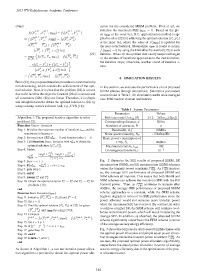
Table 1. System Parameters
Parameters Values
Algorithm.1: The proposed iterative algorithm to solve Path loss model, log 10 (ϑ) −34.5 − 38log (d[m])
10
problem (12). Corresponding distance, d 500m
Function Outer Iteration Numbers of antennas, N 4
Step 1: Initialize the maximum number of iterations i max and the Bandwidth, ∆f 10MHz
maximum tolerance ε . Noise spectral density, N 0 -174dBm/Hz
0
Step 2: Set maximum SEE η SEE = 0 and iteration index i = 0. Basic power consumption of
i
Step 3: Call Function Inner Iteration with η SEE to obtain the 40dBm
CBS, P b
i
i
optimal solution (P , P ).
c z Maximum iteration, i max 100
Step 4: Update Convergence threshold, ε 10 −3
i i
log 2 (1+ cP c )−log 2 (1+ fP i +σ 2 )
eP c
σ 2
η i+1 = c z e
SEE P c +P z +P b
i
i
Step 5: Set i = i + 1. Fig. 2 illustrates the SEE results of proposed SEEM, SR
maximization (SRM), and EE maximization (EEM) schemes
i
Step 6: if η SEE − η i−1 ≥ ε or i ≤ i max max max
SEE
Step 7: goto Step 3. versus the transmit power constraint P CBS . As P CBS increas-
Step 8: end if es, the average SEE performance of proposed SEEM and
i
i
Step 9: return P c and P z . SRM schemes all improve. This means that both SEEM and
i
i
∗
∗
Step 10: Obtain the optimal solution P c = P c and P z = P z for SRM schemes can achieve the maximum SEE with the full
max
problem (12). transmit power. Then, as P CBS continues to increase after
end 40dBm, the average SEE performance of proposed SEEM
Function Inner Iteration (η SEE) scheme approaches to a constant, while the SRM scheme
0 0 begin to degrade in terms of its SEE performance since the
0
Step 11: Initialize (P c , P z ) = (0, 0) and f = 0.
power allocator would not consume more transmit power
Step 12: Set i = 0.
when the maximum SEE has received. By contrast, in order
Step 13: Find the optimal solution (P c, P z) of (22) for given
i i to achieve a higher SR, the SRM scheme will continue to al-
(P , P ) and η SEE by using CVX.
c
z
Step 14: Compute locate more transmit power, which will result in reducing the
average SEE. In addition, as observed, the proposed SEEM
f i+1 = f 1 (P c i+1 , P z i+1 , η SEE ) − f 2 (P c i+1 , P z i+1 ).
Step 15: Set i = i + 1. scheme significantly outperforms the EEM scheme in terms
i
of the average secrecy energy efficiency.
Step 16: if f − f i−1 ≥ ε or i ≤ i max
Fig. 3 shows the SEE results of proposed SEEM scheme with
Step 17: goto Step 13.
Step 18: end if the optimal power allocation and simple equal power alloca-
max
Step 19: return P c and P z. tion strategies versus the transmit power constraint P CBS . As
end we seen, the proposed optimal power allocation significantly
outperforms the equal power allocation in terms of average
As shown in Algorithm 1, a two-tier iterative power alloca- secrecy energy efficiency, due to the optimization of the pow-
tion algorithm is provided to obtain the optimal power allo- er allocation factor.
– 144 –