Page 151 - Proceedings of the 2017 ITU Kaleidoscope

Challenges for a data-driven society

The LED Array The Lens The Imaging Plane 1
The Measured Data
0.9 The Fitting PSF Curve
(x 0 , y n-1 )
Normalizated Gray Value of The LED Image 0.6 0.5
(x 0 , y 0) 0.8 0.7
(x i , y i) 0.4
(x n-1 , y n-1) 0.3 0.2
(x n-1 , y 0 ) 0.1
0
126 225 328 450
u v Position of Pixels
(a)
Fig. 3: The optical path of the imaging light in MIMO-IS-
VLC system. 1
Diffraction light at the edge of the grating. 1 The Measured Data
0.9 The Fitting PSF Curve
2
Refraction light from the lens. 3
Reflection light on the 0.8
Normalizated Gray Value of The LED Image 0.5
inner wall of the lens’ tube. 0.7 0.6
described as the Kirk model. Establish the rectangular co- 0.4 0.3
ordinate system based on one of four corners’ LED and set 0.2
0.1
(x 0 , y 0 ) as the original point as is shown in Fig.3. Then the
0
101 225 353 450
point spread function (PSF) of the stray light is written as Position of Pixels
(b)
2
1 r i
s(r i ) = √ exp − 2 (2) 1
σ 2π 2σ 0.9 The Measured Data
The Fitting PSF Curve
0.8
p
2
2
Where r i = x + y is the distance from the point (x i , y i ) 0.7
i i
to the original point. σ is the intensity coefficient of the stray 0.6 0.5
light distribution. Assuming P(x 0 , y 0 ) is the light intensity Normalizated Gray Value of The LED Image 0.4
of the original point. Thus, to a certain area based on the cen- 0.3
ter coordinate of (x i , y i ), the stray light intensity is written 0.2
0.1
as 0 107 225 359 450
Position of Pixels
ZZ
(c)
S(x i , y i ) = K + P(x 0 , y 0 )·s(x−x i , y−y i ) dx dy (3)
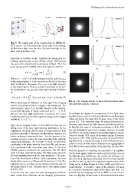
Fig. 4: The imaging results of three different lenses under
When calculating the influence of stray light in the imaging
the same photography condition.
system, the exposure time t e is ought to be considered. The
total exposure value P v is the time integral of the instanta-
R
neous light intensity P and is expressed as P v = P dt.
Because the stray light distribution function is not a time To evaluate the degree of concentration of the light inten-
correlation function, the total exposure energy can be simply sity distribution, set 0.2 as a threshold of the normalized gray
written as P v = P · t e . value and define the range that the gray value of the pixels
exceed 0.2. The narrower range the pixels distribution is,
the more concentrated the light intensity distribution will be.
Fig.4 shows imaging results of three different lens and the
In Fig.4(a), the range of horizontal coordinate is (126, 328)
fitting curve of the stray light intensity distribution. In the
that the normalized gray-value is higher than 0.2. It means
experiment, the LED and the lens of image sensor is kept
that 80% of the pixels formed by the incident light is concen-
parallel as possible to eliminate the aberrations. Analyze the
trated on around 45% pixels of the whole image. However,
pixels on image’s transversal line. For the purpose of in-
creasing accuracy, select the transversal line from different the range is (101, 353) and the proportion is around 56% in
angles and averaging. As is shown in Fig.4, he horizontal Fig.4(b) while in Fig.4c the range is (107, 359) and the pro-
coordinate is the pixels position from 0 to 450 and the ver- portion is 56% as well. It demonstrates that imaging light of
tical coordinate is the normalized gray value. A industrial the LED is more concentrative in Fig.4(a) than the other two.
CMOS camera is utilized in the experiment. The 3W white With the purpose of obtaining the parameter σ in equation
LED is at rated illumination status. The three lenses are from (2), the least square method is used to get the fitting curve of
different manufacturers with the same parameter. The diam- the light intensity distribution. As a result, the obtained σ of
eter of the three lenses is 40mm. In the experiment, the focal the curve from Fig.4(a) is 86.2 while it is 95.1 of the Fig.4(b)
length of lenses is set as 20mm and the aperture is F1.6. The and 90.2 of the Fig.4(c) (The adjusted R-square value of the
exposure time t e is 10ms and the distance from the LED to fitting curve in three images is 0.984, 0.980 and 0.985 cor-
the image sensor is 1m. The pixel size of the original image respondingly). A smaller σ value of the equation (2) leads
is 450 × 450. to a narrower distribution range of the stray light, thus it is
It can be seen that under the same photograph condition, proofed that the imaging pixel of the LED is more concen-
three lenses show difference on the imaging performance. trative in Fig.4(a). It also come to the conclusion that under

– 135 –