Page 458 - Kaleidoscope Academic Conference Proceedings 2024

2024 ITU Kaleidoscope Academic Conference

the entire image. The window slides after each
operation and the features are learnt by the
feature maps.
(N X N)* (f X f )= N – F + 1(1)
Equation 1 indicates the size of the output
matrix with no padding also known as the
feature map matrix, in this study image matrix
28*28 map 3*3 filter (28-3+1)=26, i.e. 26*26 is
the feature map. Equation 2 presents The size of
the output matrix with padding.
(NXN) * (fXf) = (N+2P–f)/(s+1)(2)
Here p is padding and s is stride. The
convolution operation is defined as Conv(m,n)
= l(x,y) ⊗ f(x,y), where ⊗ is convolution Fig6: Summary of proposed CNN Model.
operation, I(x,y) is expressing input image A specific linear process called a convolution
matrix, F(x,y) is expressing filter or kernel layer is used to extract important information.
function. So Convolution is a mathematical To reduce the covariance shift and boost neural
technique that accepts two inputs, such as an network stability, batch normalization is
image matrix and a filter or kernel. The image performed. By taking the batch mean away and
matrix is a digital representation of picture dividing it by the batch standard deviation, it
pixels, and the filter is another matrix used to normalizes the output of an earlier activation
process it. It can process any aspect of the image layer. By offering an abstracted version of the
because the kernel is significantly smaller than representation, max pooling aids in reducing
the image. This paper uses 3-by-3 filters. To be over-fitting. To avoid overfitting, the Dropout
employed in a layered architecture with layer randomly sets input units to 0 with a
numerous convolutional layers using kernels (or frequency of rate at each step during training.
filters) and a Pooling operation, each model The sum of all inputs is maintained by scaling
must first be trained, followed by testing. up non-zero inputs by 1/(1 - rate).
Rotation, Width, Height, Shear, and Zoom
variables are taken into account for data
augmentation. The accuracy of the model is
boosted when the proper values for these
parameters are filled in. As indicated in Table 2,
the CNN model's remapping parameter was
deemed false.

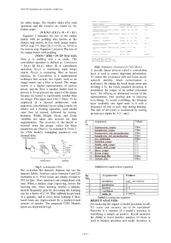
Fig 5: Architecture CNN Table2:data augmentation argument
We normalize the dataset's features but not the
dataset's labels. Feathers values between 0 and 255
normalize to 0. Pixel values are simply divided to
255 for this. Thus, machines can comprehend with
ease. When a statistic stops improving, lowers the
learning rate. Once learning reaches a plateau,
models frequently gain by decreasing the learning
rate by a factor of 2–10. This callback keeps track
of a quantity, and it slows down learning if there Table3:Learning rate argument
hasn't been any improvement for a predetermined RESULT ANALYSIS:
amount of epochs. The proposed CNN Model's For analyzing the impact of model precision, recall,
layers are depicted in Fig6. F-1 score, and accuracy are to be considered.
Precision is a measure of a model’s accuracy in
classifying a sample as positive. Recall measures
the ability to detect positive samples. F1-Score is
used to balance precision and recall. Accuracy is

– 414 –