Page 335 - Kaleidoscope Academic Conference Proceedings 2024

Innovation and Digital Transformation for a Sustainable World

The LDPC codes were invented by R. Gallager in 1963 [9]. ℋ + ℋ + ⋯ + ℋ = 0, where [ℋ ℋ … ℋ ] are

1 1

2 2
2
1
An LDPC code consists of combinations of repetition codes the columns of the matrix ℋ . This shows that is the
(RC) and single parity check (SPC) codes. The number kernel of ℋ and this is known as the kernel representation.
number of edges coming out at the SPC are equal to the
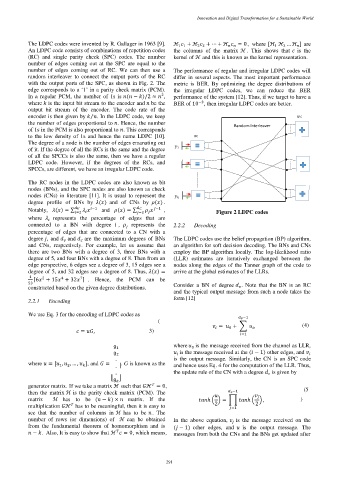
number of edges coming out of RC. We can then use a The performance of regular and irregular LDPC codes will
random interleaver to connect the output ports of the RC differ in several aspects. The most important performance
with the output ports of the SPC, as shown in Fig. 2. The metric is BER. By optimizing the degree distributions of
edge corresponds to a ‘1’ in a parity check matrix (PCM). the irregular LDPC codes, we can reduce the BER
In a regular PCM, the number of 1s is ( − )/2 ≈ , performance of the system [12]. Thus, if we target to have a
2
where is the input bit stream to the encoder and be the BER of 10 , then irregular LDPC codes are better.
−3
output bit stream of the encoder. The code rate of the
encoder is then given by . In the LDPC code, we keep SPC
⁄
the number of edges proportional to . Hence, the number
Random Interleaver
of 1s in the PCM is also proportional to . This corresponds
to the low density of 1s and hence the name LDPC [10]. RC
The degree of a node is the number of edges emanating out
of it. If the degree of all the RCs is the same and the degree
of all the SPCCs is also the same, then we have a regular
LDPC code. However, if the degrees of the RCs, and
SPCCs, are different, we have an irregular LDPC code.
The RC nodes in the LDPC codes are also known as bit
nodes (BNs), and the SPC nodes are also known as check
nodes (CNs) in literature [11]. It is usual to represent the
degree profile of BNs by ( ) and of CNs by ( ) .
−1 −1
Notably, ( ) = ∑ and ( ) = ∑ ,
=2 =2 Figure 2 LDPC codes
where represents the percentage of edges that are

connected to a BN with degree , represents the 2.2.2 Decoding

percentage of edges that are connected to a CN with a
degree , and and are the maximum degrees of BNs The LDPC codes use the belief propagation (BP) algorithm,

and CNs, respectively. For example, let us assume that an algorithm for soft decision decoding. The BNs and CNs
there are two BNs with a degree of 3, three BNs with a employ the BP algorithm locally. The log-likelihood ratio
degree of 5, and four BNs with a degree of 8. Then from an (LLR) estimates are iteratively exchanged between the
edge perspective, 6 edges see a degree of 3, 15 edges see a nodes along the edges of the Tanner graph of the code to
degree of 5, and 32 edges see a degree of 8. Thus, ( ) = arrive at the global estimates of the LLRs.
1 2 4 7
[6 + 15 + 32 ] . Hence, the PCM can be
53 Consider a BN of degree . Note that the BN is an RC
constructed based on the given degree distributions.
and the typical output message from such a node takes the
form [12]
2.2.1 Encoding
We use Eq. 3 for the encoding of LDPC codes as
−1
(
= + ∑ , (4)
0

= , 3)
=1
1 where is the message received from the channel as LLR,
0
2 is the message received at the ( − 1) other edges, and

. is the output message. Similarly, the CN is an SPC code
where = [ , , … , ], and = . . G is known as the and hence uses Eq. 4 for the computation of the LLR. Thus,

1
2

. the update rule of the CN with a degree is given by

[ ]

generator matrix. If we take a matrix ℋ such that ℋ = 0, (5
then the matrix ℋ is the parity check matrix (PCM). The −1

matrix ℋ has to be ( − ) × matrix. If the ℎ ( ) = ∏ ℎ ( ) , )
multiplication ℋ has to be meaningful, then it is easy to 2 =1 2

see that the number of columns in ℋ has to be . The
number of rows (or dimensions) of ℋ can be obtained In the above equation, is the message received on the

from the fundamental theorem of homomorphism and is ( − 1) other edges, and is the output message. The

− . Also, It is easy to show that ℋ = 0, which means, messages from both the CNs and the BNs get updated after
– 291 –