Page 206 - Kaleidoscope Academic Conference Proceedings 2021

2021 ITU Kaleidoscope Academic Conference

different network load scenarios representing a light and
heavy network traffic to simulate the traffic variations along
with the scenes. The simulation alternates light and heavy
traffic in each 1000 scenes. The total throughput of the
heavy scenario is bigger than the lighter one. Each user
has a specific traffic magnitude defined as a percentage of
total throughput in accordance with Table 1, enabling the
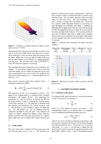
differentiation of applications. Figure 6 shows the histogram
of traffic throughput for each user in Gbps. Each user presents
the heavy and light traffic behavior. The incoming traffic for
each user is buffered when there is buffer space available,
otherwise the excess of packets are tail-dropped. The packets
are also dropped when they occupy the buffer for more than
10 seconds.
Table 1 – Network load information for light and heavy
scenarios.
Figure 5 – Example of radiation pattern for specific beam
index with an 8 × 8 UPA. Network load Total throughput UAV (%) Pedestrian (%) Car (%)
Light 0.48 Gbps 50% 20% 30%
channel model [16]. The reason for this choice is that we first Heavy 0.96 Gbps 50% 20% 30%
want to evolve the AI/ML engine such that newer versions
allow rendering in (near) real-time, along the training of the
RL agent. Right now, we are not able to render each scene
and the agent choices, but CAVIAR-v2 is being developed
with this goal. We will later work in the CAVIAR-RT-v1,
where RT stands for support to ray tracing.

The simplified H currently represents a Line-of-Sight (LoS)
channel. A narrowband channel model [16] is used, but
wideband models can be readily incorporated in case their
extra computational cost is not an issue. For simplicity, the
users have a single antenna (N r = 1) while the BS has a 8 × 8
UPA (N t = 64).

The geometric channel model [16] is adopted with L = 2 Figure 6 – Histogram of packets traffic received by the BS
Multipath Components (MPCs): for each user.

p L Õ A A ∗ D D
H = N t N r α ` a r (φ , θ )a (φ , θ ). (3)
t
` ` ` ` 4. MACHINE LEARNING MODEL
`=1
The parameters in Eq. (3) are obtained as follows. The 4.1 Evaluation of RL agents
phase of the complex-gain α ` is obtained from a uniform
To evaluate the RL agent, the return G over the test episodes
distribution with support [0, 2π]. For generating the
is used. The return G e for episode e is
magnitude |α ` |, first the distance d between the BS and
the given receiver is used to calculate the received power N s e
Õ
via the Friis equation [17]. The path loss is obtained from G e = r e [t], (4)
this equation and determines |α ` |, which decreases with t=1
d. The elevation φ ` and azimuth θ ` angles, for departure where N e is the number of scenes in episode e. The
A
D
(e.g. φ ) and arrival (e.g. φ ) are obtained from the s
corresponding reward r e [t] at discrete-time t is a weighted
` `
orientation provided by the LoS path. The nominal LoS
sum of transmitted and discarded packets given by
angles are slightly changed by adding to them Gaussian
random variables with zero-mean and variance of 1 degree. P tx [t] − 2P d [t]
r e [t] = (5)
These angles are used to compose the steering vectors a t and P b [t] ,
a r .
where P tx [t], P d [t], and P b [t] correspond, respectively, to the
total amount (summation for all users) of transmitted, dropped
3.1 Traffic model and buffered packets at time t. The reward r e [t] is restricted
to the range −2 ≤ r e [t] ≤ 1. At each time t, a single user can
The users’ data traffic is defined as Poisson processes with be served, but P b [t] accounts for the number of packets in all
time-varying mean λ u [t] for user u. We specified two three buffers. Hence, r e [t] = 1 only if all buffered packages

– 144 –