Page 79 - ITU Journal Future and evolving technologies Volume 2 (2021), Issue 4 – AI and machine learning solutions in 5G and future networks

ITU Journal on Future and Evolving Technologies, Volume 2 (2021), Issue 4

sponding hidden states of the link (ℎ ) and the path

(ℎ ), and introduce this as input of the readout function.

Thus, the resulting weight , can be interpreted as
quantifying the importance for RouteNet of a particular
src‑dst path as it passes through a certain link of the
network.

6.2 Evaluation of the accuracy

We evaluate the accuracy achieved by the NetXplain
model on samples simulated in three real‑world topolo‑
gies [18]: NSFNet (14 nodes), GEANT2 (24 nodes), and
GBN (17 nodes). Concretely, for each topology we ran‑
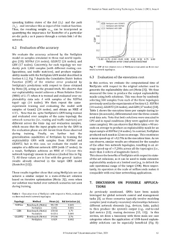
Fig. 7 – CDF of the relative error of NetXplain evaluated on three real‑
domly pick 1,000 samples (with different routing con‑
world network topologies.
igurations, and ic matrices), and produce explain‑
ability masks with the NetXplain GNN model described in
6.3 Evaluation of the execution cost
Section 6.1.2. Fig. 7 depicts the Cumulative Distri‑ bution
Function (CDF) of the relative error produced by In this section, we evaluate the computational time of
NetXplain’s predictions with respect to those obtained
NetXplain with respect to the original solution used to
by Metis [3], acting as the ground truth. We observe that
generate the explainability data set (Metis [3]). We thus
our explainability model achieves a Mean Relative Error
measured the time to produce the output explainability
(MRE) of 2.4% when it is trained and evaluated over ex‑
masks using both solutions. This was done by randomly
plainability data sets with samples of the NSFNet
selecting 500 samples from each of the three topologies
topol‑ ogy (14 nodes). We then repeat the same previously used in the experiments of Section 6.2: NSFNet
experiment training and evaluating the model with
(14 nodes), GEANT2 (24 nodes), and GBN (17 nodes) [18].
samples of Geant2 (24 nodes), and obtain an MRE of
Table 1 shows the execution times per sample during in‑
4.5%. Note that de‑ spite NetXplain’s GNN being trained
ference (in seconds), differentiated over the three consid‑
and evaluated over samples of the same topology, the
ered data sets. Note that both solutions were executed in
network scenarios (i.e., routing and traf ic matrices) are
CPU and in equal conditions (they were applied over the
different across the train‑ ing and evaluation samples,
same samples). We can observe that Metis takes ≈98 sec‑
which means that the input graphs seen by the GNN in
onds on average to produce an explainability mask for an
the evaluation phase are dif‑ ferent from those observed
input sample of NSFNet (14 nodes). In contrast, NetXplain
during training. Finally, we further test the
produced each mask in 12 ms on average. This constitutes
generalization capabilities of NetXplain by training the
a mean speed‑up of ≈8,178x in the execution time. As we
explainability GNN with samples from NSFNet and
can observe, similar results are obtained for the samples
GEANT2, but in this case, we evaluate the model on
of the other two network topologies, resulting in an av‑
samples of a different network: GBN (with 17 nodes). As
erage speed‑up of ≈7,200x across all the topologies (i.e.,
a result, NetXplain achieves an MRE of 11%over this more than 3 orders of magnitude faster).
network topology unseen in advance (dashed line in Fig.
This shows the bene its of NetXplain with respect to state‑
7). All these values are in line with the general‑ ization
of‑the‑art solutions, as it can be used to make extensive
results already observed in the target GNN model explainability analysis at a limited cost (e.g., to delimit the
(RouteNet [12]).
safe operational range of the target GNN). More impor‑
tantly, its operation at the scale of milliseconds makes it
These results together show that using NetXplain we can compatible with real‑time networking applications.
achieve a similar output to a state‑of‑the‑art solution
based on iterative optimization (Metis [3]), even when
our solution was tested over network scenarios not seen 7. DISCUSSION ON POSSIBLE APPLICA‑
during training. TIONS
As previously mentioned, GNNs have been mainly
Table 1 – Execution time of NetXplain with respect to Metis, evaluated leveraged for global network control and management
on three real‑world network topologies
tasks [3], as these scenarios typically involve modeling
Topology Method Mean (s) Std deviation (s) complex (and mutually recursive) relationships between
NSFNet Benchmark (Metis) 98.139 2.455 different network elements (e.g., devices, links, paths)
NetXplain 0.012 0.001 to then produce the system’s output (e.g., end‑to‑end
GBN Benchmark (Metis) 150.83 1.79 QoS metrics [12], routing decisions [15, 13]). In this
NetXplain 0.0214 0.005
GEANT2 Benchmark (Metis) 191.46 2.76 section, we draw a taxonomy with three main use case
NetXplain 0.029 0.002 categories where the application of GNN‑based explain‑
ability solutions can be especially bene icial (Fig. 8):
© International Telecommunication Union, 2021 63