Page 76 - ITU Journal Future and evolving technologies Volume 2 (2021), Issue 4 – AI and machine learning solutions in 5G and future networks

ITU Journal on Future and Evolving Technologies, Volume 2 (2021), Issue 4

Note that when applying GNN to network‑related prob‑
lems, input graphs may contain a wide variety of el‑
ements and connections that do not necessarily corre‑
spond to physical network elements (e.g., forwarding de‑
vices, links). For instance, some proposals like [12, 16]
introduce complex hypergraphs including logic network
entities (e.g., end‑to‑end paths).
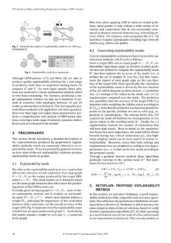
Fig. 3 – Schematic description of explainability solutions for GNN (e.g.,
GNNExplainer)
4.2 Generating explainability masks
Current explainability solutions are based on iterative op‑
timization methods, which work as follows:
Given a target GNN and an input graph = ( , ), ex‑
plainability algorithms apply an iterative (costly) gradi‑
ent descent method to compute the explainability mask
Fig. 4 – Explainability mask of an input graph.
that best explains the accuracy of the model (i.e., it
de ines the set of weights (see Eq. (5))) that repre‑
Although GNNExplainer [17] and Metis [3] are able to
sents the impact of each graph edge on the loss func‑
produce quality explainability solutions for a vast range
tion of the target GNN. More speci ically, the calculation
of problems, both have an important limiting factor. To
′ ′ of the explainability mask is driven by the loss function
compute and for each input sample, these solu‑
of Eq. (6), which depends on three factors: ( ) predictive
tions use an iterative convex optimization method, which
loss, ( ) entropy of the values in the mask, and ( ) L1
is very time‑consuming. For instance, producing a sin‑
regularization computed over the mask. The predictive
gle explainability solution can take up to hundreds of sec‑
loss quanti ies how the accuracy of the target GNN ( )
onds in scenarios with topologies between 14 and 24
degrades when weighting the hidden states according to
nodes, as shown later in Section 6. This fact arguably pre‑
( ). Note that the predictive loss function greatly de‑

vents these methods to be applied for real‑time operation.
pends on the speci ic problem we aim to solve (e.g., re‑
Moreover, their high cost makes them impractical to per‑
gression or classi ication). The entropy factor (Eq. (7))
form a comprehensive test analysis of GNN‑based solu‑
controls the trade‑off between too homogeneous or too
tions, covering a wide range of network scenarios, before sparse values in the resulting mask . Finally, the 1
these tools are released to the market.
regularization controls the number of connections that
will have high values. More in detail, as the regulariza‑
4. PRELIMINARIES tion factor has more importance, the mask will be driven
towards having less critical connections (i.e., less high‑
This section irstly introduces a detailed description of value weights), which can be more useful for human in‑
the representations produced by graph‑based explain‑ terpretability. Moreover, notice that both entropy and
ability methods, which are commonly referred to as ex‑ regularization loss are weighted according to two hyper‑
plainability masks. Then, we present the general overview parameters (i.e., , ) that can be ine‑tuned according to
on how state‑of‑the‑art explainability solutions produce the problem’s needs.
explainability masks on graphs. Through a gradient descent method, these algorithms
∗
gradually converge to the optimal mask that mini‑
4.1 Explainability mask mizes the loss function ℓ( ).
We refer to the explainability mask as an n×n matrix that ℓ( ) = ( , ) + ( ) + || || 1 (6)

de ines the relevance of each connection of an input graph
( ) = − ∑( , log( ) + (1 − ) log(1 − )) (7)
,
,
,
= ( , ) on the output produced by the target GNN,
,
where = | |. This mask enables us to interpret which
are the main graph elements that affect most the predict‑ 5. NETXPLAIN: PROPOSED EXPLAINABILITY
ing power of the GNN in each case.
Formally, given an input graph = ( , ), state‑of‑the‑ METHOD
art explainability methods aim to produce an explainabil‑ In this section, we introduce NetXplain, a novel explain‑
ity mask ∈ {0, 1} × , where each element de ines a ability method for GNN, compatible with real‑time opera‑
weight , indicating the importance of the connection tions, that addresses the performance limitations of exist‑
between node and node on the overall accuracy of the ing solutions (Section 3). NetXplain is able to produce the
target GNN. Fig. 4 illustrates how the explainability mask same output as state‑of‑the‑art solutions, based on costly
is built from an input (undirected) graph . Particularly, iterative optimization algorithms [17, 3], while operating
this matrix contains a weight for each pair ( , ) connected at a much limited cost (at the scale of a few milliseconds
in the graph. in our experiments in Section 6). This not only enables us

60 © International Telecommunication Union, 2021