Page 127 - ITU Journal Future and evolving technologies Volume 2 (2021), Issue 3 – Internet of Bio-Nano Things for health applications

ITU Journal on Future and Evolving Technologies, Volume 2 (2021), Issue 3

Evolutionary game theory is a two‑stage process. In the the total number of dropped messages or maximize the total
irst stage, the population members undergo a selection number of transmissions. Note that there might be other
process depending on the individual strategies of the communication‑related goals such as faster communica‑
pop‑ ulation. In the second stage, selected individuals tion or communicating with fewer resources, however,
create new offspring. The phases of evolutionary game for the sake of simplicity, we only focus on the maximum
theory are depicted in Fig. 4. number of dropped messages from sensor nodes to the
sink for this problem. As a result, organisms with a lower
In this section, we irst describe the toy problem and then
number of drops are selected to create offspring. Since
present an analytic solution using the simple geometry of
we consider the organisms individually, we assume they
the toy problem. Then, we demonstrate an evolutionary do not interact with each other.
solution for the same problem and compare the results
with the analytic solution. Without loss of generality, we assume that sensor nodes
have unlimited resources, i.e., they safely outlast the relay
3.1 Problem description nodes. Without this assumption, dried‑up sensor nodes
might stop creating messages before relay nodes stop
transmitting them. Hence, such an assumption helps us
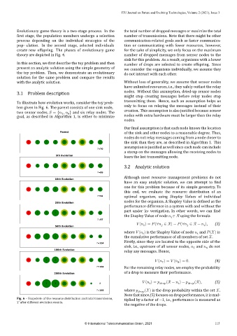
To illustrate how evolution works, consider the toy prob‑
lem given in Fig. 6. The parent consists of one sink node, only to focus on relaying the messages instead of their
creation. This assumption is also justi ied because sensor
two sensor nodes, = { , } and six relay nodes. The
6
4
goal, as described in Algorithm 1, is either to minimize nodes with extra hardware must be larger than the relay
nodes.
Our inal assumption is that each node knows the location
of the sink and other nodes to a reasonable degree. Thus,
Parent
nodes do not relay messages coming from a node closer to
0 1 2 3 4 5 6 7 8 the sink than they are, as described in Algorithm 1. This
assumption is justi ied as well since each node can include
T
a stamp on the messages allowing the receiving nodes to
learn the last transmitting node.
5th Evolution
3.2 Analytic solution
0 1 2 3 4 5 6 7 8
T
Although most resource management problems do not
10th Evolution
have an easy analytic solution, we can attempt to ind
one for this problem because of its simple geometry. To
0 1 2 3 4 5 6 7 8
this end, we evaluate the resource distribution of an
optimal organism, using Shapley Values of individual
T
nodes for the organism. A Shapley Value is de ined as the
20th Evolution
performance difference in a system with and without the
part under in‑ vestigation. In other words, we can ind
0 1 2 3 4 5 6 7 8
the Shapley Value of node ∈ ℛ using the formula

T
( ) = (∀ ∈ ℛ) − (∀ ∈ ℛ − ), (3)

50th Evolution
where ( ) is the Shapley Value of node and ( ) is

0 1 2 3 4 5 6 7 8 the cumulative performance of all members of set .
Firstly, since they are located to the opposite side of the

T
sink, i.e., upstream of all sensor nodes, and do not
7
8
relay any messages. Hence,
100th Evolution
0 1 2 3 4 5 6 7 8 ( ) = ( ) = 0. (4)
8
7
T For the remaining relay nodes, we employ the probability
of a drop to measure their performance.
200th Evolution
( ) = (ℛ − ) − (ℛ), (5)
0 1 2 3 4 5 6 7 8
where ( ) is the drop probability within the set .
T
Note that since (5) focuses on drop performance, it is mul‑
Fig. 6 – Snapshots of the resource distribution and total transmission, tiplied by a factor of −1, i.e., performance is measured as
after different evolution counts.
the negative of the drops.
© International Telecommunication Union, 2021 115