Page 50 - ITU Journal, ICT Discoveries, Volume 3, No. 1, June 2020 Special issue: The future of video and immersive media

ITU Journal: ICT Discoveries, Vol. 3(1), June 2020

based cluster was used for measuring decoder runtimes. diction residual res. Thus, at the decoder, one can re-
No SIMD- or GPU-based optimization was applied. Ac- place the computation of T −1 (c) by the computation of
cording to the architecture of the neural-networks used, T −1 (c+pred i,tr ). Consequently, as long as the prediction
the total number of parameters needed for the prediction residual is non-zero, no extra inverse transform needs to
modes described in this section is about 5.5 million. Since be executed when passing from pred i,tr to pred i .
all parameters were stored in 16-bit-precision, this corre- The weights θ i of the involved neural-networks were ob-
sponds to a memory requirement of about 11 Megabyte. tained in two steps. First, the same training algorithm
Our method should be compared to the method of [16], as in the previous section was applied and the predictors
where also intra-prediction modes based on fully con- were transformed to predict into the frequency domain.
nected layers are trained and integrated into HEVC. While Then, using again a large set of training data, for each pre-
the compression benefit reported in [16] is similar to dictor it was determined which of its frequency compo-
ours, its decoder runtime is significantly higher; see Ta- nents could be set to zero without significantly changing
ble III of [16]. its quality on natural image content. For more details, we
refer to [14].
4. PREDICTIONINTOTHETRANSFORMDO- As a further development, for the signalization of con-
MAIN ventional intra-prediction modes, a mapping from neural-
network-based intra-prediction modes to conventional
The complexity of the neural-network-based intra- intra-prediction modes was implemented. Via this map-
prediction modes from the previous section increases ping, whenever a conventional intra-prediction mode is
with the block-sizes W and H. This is particularly true used on a given block, neighboring blocks which use the
for the last layer of the prediction modes, where for each neural-network-based prediction mode can be used for
output sample of the final prediction, 2 · (W + H + 2) the generation of the list of most probable modes on the
many multiplications have to be carried out and a given block. For further details, we refer to [14].
(W · H) × (2 · (W + H + 2))-matrix has to be stored for In an experimental setup similar to the one of the pre-
each prediction mode. vious section, the intra-prediction modes of the present
Thus, instead of predicting into the sample domain, in section gave a compression benefit of −3.76% luma-BD-
subsequent work [21, 14] we transformed our predictors rate gain; see [14, Table 2]. Compared to the results of the
such that they predict into the frequency domain of the previous section, these results should be interpreted as
discrete cosine transform DCT-II. Thus, if T is the matrix saying that the prediction into the transform-domain with
representing the DCT-II, the i-th neural-network predic- the associated reduction of the last layer does not yield
any significant coding loss and that the mapping from
tor from the previous section predicts a signal pred i,tr
such that the final prediction signal is given as neural-network-based intra-prediction modes to conven-
tional intra-prediction modes additionally improves the
−1
pred i = T · pred i,tr .
compression efficiency. As reported in [14], the mea-
sured decoder runtime overhead is 147%, the measured
The key point is that each prediction mode has to follow a
fixed sparsity pattern: For a lot of frequency components, encoder runtime overhead is 284%. Thus, from a de-
coder perspective, the complexity of the method has been
pred i,tr is constrained to zero in that component, inde-
significantly reduced. Also, the memory requirement of
pendent of the input. In other words, if A i,tr is the matrix
the method was reduced significantly. In the architecture
used in the last layer for the generation of pred i,tr , then
from Figure 5, approximately 1 Megabyte of weights need
for each such frequency component, the row of the ma-
to be stored.
trix A i,tr corresponding to that component consists only
of zeros. Thus, the entries of that row do not need to be
stored and no multiplications need to be carried out in the 5. MATRIX-BASED INTRA-PREDICTION
matrix vector product A i,tr i · ftr for that row. The whole MODES
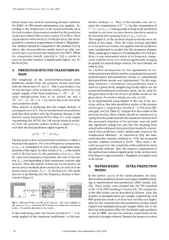
process of predicting into the frequency domain is illus-
In the further course of the standardization, the data-
trated in Figure 5.
driven intra-prediction modes were again simplified lead-
ing to matrix-based intra-prediction (MIP) modes, [23,
26]. These modes were adopted into the VVC-standard
at the 14-th JVET-meeting in Geneva [9]. The complexity
of the MIP modes can be described as follows. First, the
number of multiplications per sample required by each
MIP-prediction mode is at most four and thus not higher
Fig. 5 – intra-prediction into the DCT-II domain. The white samples in than for the conventional intra-prediction modes which
the output pred i,tr denote the DCT-coefficients which are constrained require four multiplications per sample either due to the
to zero. The pattern depends on the mode i.
four-tap interpolation filter for fractional angle positions
In the underlying codec, the inverse transform T −1 is al- or due to PDPC. Second, the memory requirement of the
ready applied to the transform coefficients c of the pre- method is strongly reduced. Namely, the memory to store

28 © International Telecommunication Union, 2020