Page 105 - Proceedings of the 2018 ITU Kaleidoscope

Machine learning for a 5G future

percentage of received data, for all the applications obtaining 1 No policy
the final performance index value D. In order to observe Deep RL
the index after the action execution, we wait for ten seconds. 0.8
Depending on the difference between the indexes evaluated
before and after the execution on an action in the environment,
we were able to define the reward as a number r which 0.6
can assume the following values: [-1,-2/3,-1/3,0,1/3,2/3,1] Percentage of received data - D
where a value nearby one means that the action performed 0.4
resulted in an improvement of system performance while a
value nearby minus one means that the action performed
resulted in a decrease of the system performance. For the 0.2
sake of simplicity, we considered that UEs can only run one
application per time. Our goal is to produce an optimal
policy, which is able to address the problem related to the 0 100 200 300 400
user’s mobility inside the network in order to improve user Simulation time (sec)
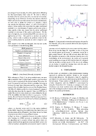
QoS. Figure 5 – Comparison between the performance obtained by
With respect to the DNN we designed, here we sum up the the Deep RL policy and a scenario where the data migration
main parameters in the following table: is not enabled.
DNN parameters maintain in both simulation the same user mobility pattern.

Number o f hidden layers 3 Plots show that the Deep RL algorithm is able to improve
the overall system performance, in particular except for a
Number o f neurons 15
little period between 100 and 200 seconds where the Deep
Input dimension 21 RL algorithm encounters a little decrease (mainly due to the
Output dimension 9 stochasticity of the environment), the results are in general
Learning rate 0.001 good reaching an average of 0.60 which is better if compared
with the no policy average equal to 0.54. As we are writing,
Activation f unction ReLU
we are trying to extend the training time with the aim to
Update step 50 further improve the obtained results.
Batch size 32
Experience replay dimension 2000 6. CONCLUSIONS
In this paper, we presented a deep reinforcement learning
Table 2 – Deep Neural Network parameters.
approach to address the problem related to the network
With reference to Table 2, by doing multiple tests, we were environment dynamics. We designed a Deep RL algorithm
able to establish that 3 hidden layers create a good topology and tested it in a real scenario demonstrating the feasibility of
which is able to properly fit the desired output. Moreover, we the technique. Future works will be devoted to implement
fixed 15 neurons for each layer which is a number that stays in a better integration with the OMNeT++ environment by
between the input layer dimension and the output one. With using the Tensorflow C++ frontend, to compare with other
respect to the activation function, we used the Rectified Linear solutions,to use more realistic traffic and mobility models,
Unit (ReLU) which resulted in a faster learning if compared and to the investigation of new indexes with the aim to further
with other functions like the sigmoid. Since our DNN has to improve the system performance.
predict the state Q-values which are values defined in the set
of R, the problem we tried to solve is a regression. For this REFERENCES
reason, the cost function we used is the Mean Squared Error [1] D. Bruneo, S. Distefano, F. Longo, G. Merlino, and
(MSE) which is typical for this kind of problems and defined
as: A. Puliafito, “I/Ocloud: Adding an IoT Dimension to
Cloud Infrastructures,” Computer, vol. 51, no. 1, pp.
1 n Õ 2
MSE = (y i − by i ) (12) 57–65, January 2018.
n
i [2] R. Dautov, S. Distefano, D. Bruneo, F. Longo,
where y is the real output and by i is the output predicted G. Merlino, and A. Puliafito, “Data processing
by the DNN. Regarding the update step, the batch size, and in cyber-physical-social systems through edge
the experience replay dimension, the values we set has been computing,” IEEE Access, vol. 6, pp. 29822–29835,
obtained empirically by trying different values. 2018.
In Fig.5 we show a comparison between the policy learned
after training for 25000 seconds of simulation our Deep [3] P. Bellavista, A. Zanni, and M. Solimando, “A
RL algorithm and a scenario without any policy where we migration-enhanced edge computing support for mobile
simply distributed one application for each MEC server. For devices in hostile environments,” in 2017 13th
a fair comparison, we used the same random seed in order to International Wireless Communications and Mobile

– 89 –