
Page 102 - Proceedings of the 2018 ITU Kaleidoscope
P. 102
2018 ITU Kaleidoscope Academic Conference
Q values in the update rule which can be expressed as follows:
y j,a = r j + γ max(Q(s j+1 , θ)) (4)
b
b
where y j,a is the Q-value associated to the state j when
the agent performs the action a,r j is the reward associated
to the state s j , and Q(s j+1 , θ) is the output layer of target
b
b
DNN network which contains the Q-values estimation for the
state s j+1 . By using two networks instead of just one, the
obtained result is a more stable training which is not affected
by learning loops due to the self-update network targets that
sometimes can lead to oscillations or policy divergence.
3.2 Problem Formulation
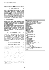
Algorithm 1: Deep RL
In order to properly design a deep RL algorithm, it is first of 1 initialize experience replay memory E to {}
all necessary to define the environment in which the RL agent 2 random initialize main DNN network weights θ
will operate. In this subsection, we will formalize the MEC
b
3 set target DNN network weights θ equal to θ
scenario we are interested in.
4 set discount factor γ
We start defining as N the number of eNBs present in the 5 set batch size
MEC-enabled LTE network. For the sake of simplicity and 6 set update step U
without loss of generality, let us assume that to each eNB is 7 set waiting time t
attached one and only one MEC server. Then, let us define 8 set exploration rate
the set, with cardinality N ∈ N, of the MEC servers attached 9 set decay rate d
to the eNBs as: 10 for episode = 1 to end:
11 observe current state s j
MEC = [MEC 1 , MEC 2 , MEC 3 , ..., MEC N ] (5) 12 p = random([0,1])
13 if > p:
Users are free to move around the MEC environment 14 action = random([1,Z])
and attach to different eNBs through seamless handover 15 else:
procedures. Moreover, they run several applications whose 16 action = argmax(Q(s j ,θ))
data is contained in the Cloud or inside one of the MEC 17 end if
servers. Regarding the applications that users can run and the 18 execute the action
number of devices attached to the eNBs, we can define the 19 wait(x seconds)
following sets: 20 observe the new state s j+1
21 observe the reward r
Apps = [app 1 , app2, app 3 , ..., app M ] (6) 22 store the t-uple (s j ,action,s j+1 ,r) in E
23 sample a batch from E
Devices = [UE 1 , UE 2 , UE 3 , ..., UE K ] (7) 24 y = Q(s j ,θ)
y target = Q(s j+1 ,θ)
25
with M, K ∈ N. With respect to the actions that the agent can y action = r + γ · max(y target )
b
b
perform in the environment, let us define the set of actions 26 execute one training step on main DNN network
with cardinality Z ∈ N as: 27
28 every U steps set θ = θ
b
Actions = [a 1 , a 2 , a 3 , ..., a Z ] (8) 29 end for
where each element represents an app migration from the
Cloud towards one of the servers defined in the MEC set,
from one MEC server to the Cloud, or among MEC servers.
Another important element that we have to introduce is the
concept of state which is made of a t-uple containing all
the information related to the users position and the app
distribution over the network which is defined as follows:
(9)
s =< (s 1 , s 2 , s 3 , ..., s T ) >
Finally, with respect to the reward, we define it as a number
r ∈ R that is computed as a combination of several network
performance indexes.
– 86 –