Page 98 - ITU Journal - ICT Discoveries - Volume 1, No. 2, December 2018 - Second special issue on Data for Good

ITU JOURNAL: ICT Discoveries, Vol. 1(2), December 2018

structure, a bell fuzzy axon with the bell-shaped From reference [23], the output of fuzzy axon is
curve as its MF was applied to the input calculated using equation (13):
telecommunication network traffic variable, hourly,
daily, weekly, monthly and quarterly respectively as ݂ ሺݔǡ ݓሻ ൌ݉݅݊׊ ቀܯܨ൫ݔ ǡݓ ൯ቁ ሺͳ͵ሻ
௜
௝
௜
௜௝
shown in equation (12). The fuzzy axon has the
advantage of modifying the MF while the network where, i = input index, j = output index, ݔ = input i,
௜
training process continues over back propagation ݓ = weights (MF parameters) corresponding to
௜௝
which ensures convergence. The MFs per input used the jth MF of input i and MF is the membership
were 3. function of the particular subclass of the fuzzy axon.
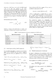
Bell function is given as [20]: The parameters applied for configuring the
ͳ network are grouped under input and output as
ߤ ሺݔሻ ൌ ଶ௕ ೔ ሺͳʹሻ shown in Table 1. The momentum algorithm was
ଵ
ଵ
ͳ൅ฬ ሺݔ െ ܿ ሻ ฬ chosen as the learning rule with the axon as the
ܽ
ଵ
transfer function. The fuzzy model reasoning
approach of the Tsukamoto model and the Sugeno
model (TSK) were implemented.
where x = input to the node and a1, b1 and c1 are
adaptable variables known as premise parameters.

Table 1 – Network parameter selection for configuration of CANFIS model

Input layer parameter Output layer parameters
Input PE 5 Transfer function Axon
Output PE 5 Learning rule Momentum
Exemplars 271 Step size 1
Hidden layer 0 Momentum 0.7
Membership function Bell Maximum epochs 1000
MFs per input 3 Termination MSE (Increase)
Fuzzy model TSK Weight update Batch

ݐ݄݁݊ ݑ ௠ ൌ ݌ ௠ଵ ଵ ௠ଶ ଶ ௠௡ ௡
ݖ ൅݌
ݖ ൅ڮ ൅݌
ݖ ൅
2.3 Initialization of the CANFIS network ݍ ሺͳ͸ሻ
௠
For a model initialization, a common rule set with n 2.4 Prediction measure of accuracy
input and m IF-THEN rules are used in equation
(14), equation (15) and equation (16) as follows In order to determine the goodness of fit of the
[23]: CANFIS models the following statistical measures
are used as shown mathematically in equation (17),
equation (18)
ܴݑ݈݁ ͳǣ ܫ݂ ݖ ݅ݏ ܣ ܽ݊݀ ݖ ݅ݏ ܣ ଵଶ ǥܽ݊݀ ݖ ݅ݏ ܣ ଵ௡ and equation (19). A model with a
ଶ
ଵ
௡
ଵଵ
minimum value is selected for forecasting.
ݖ
ݐ݄݁݊ ݑ ൌ ݌ ݖ ൅݌ ݖ ൅ڮ ൅݌ ଵ௡ ௡
ଵଶ ଶ
ଵ
ଵଵ ଵ
൅ݍ ሺͳͶሻ Mean squared error (MSE) is calculated as:
ଵ
ܴݑ݈݁ ʹǣ ܫ݂ ݖ ݅ݏ ܣ ܽ݊݀ ݖ ݅ݏ ܣ ଶଶ ǥܽ݊݀ ݖ ݅ݏ ܣ σ ௉ିଵ ேିଵ ሺ݀ െݕ ሻ ଶ
σ
ଵ
ଶ௡
ଶଵ
ଶ
௡
ܯܵܧ ൌ ௝ୀ଴ ௜ୀ଴ ܰܲ ௜௝ ௜௝ ሺͳ͹ሻ
ݐ݄݁݊ ݑ ൌ ݌ ݖ ൅݌ ݖ ൅ڮ ൅ ݌ ଶ௡ ௡
ݖ
ଶ
ଶଶ ଶ
ଶଵ ଵ
൅ݍ ሺͳͷሻ Normalised root mean squared error (NRMSE) is
ଶ
given as:
ڭ ξܯܵܧ
ܴݑ݈݁ ݉ǣ ܫ݂ ݖ ݅ݏ ܣ ௠ଵ ܽ݊݀ ݖ ݅ݏ ܣ ௠ଶ ǥܽ݊݀ ܴܰܯܵܧ ൌ ݉ܽݔ൫݀ ൯െ݉݅݊൫݀ ൯ ሺͳͺሻ
ଵ
ଶ
σ ௉ିଵ ௜௝ ܲ ௜௝
௝ୀ଴
ݖ ݅ݏ ܣ ௠௡
௡
76 © International Telecommunication Union, 2018