Page 53 - ITU Journal Future and evolving technologies Volume 3 (2022), Issue 2 – Towards vehicular networks in the 6G era

ITU Journal on Future and Evolving Technologies, Volume 3 (2022), Issue 2

An iterative updating method for position, called desired positions given by the green arrows, taking
the Gradient-Based-Mobility-Updating (GBMU) the trade-off of PRR vs fairness.
algorithm, is proposed to move a broadcast The availability of the parameters in GBMU:
transmitter i and it consists of five steps:
Throughout steps 1-5, our GBMU algorithm
• Step 1: Transmitter i obtains gradient ( ) requires the transmitter to know for each j, a) the
,
of the current iteration k for all target receivers position of j, b) the position of the main interferer of
j by: j, c) Number of Surrounding interfering Vehicles
1 1 (NSVs) so that the associated coefficient values to
( ) = ∙ , ( ) ∙ , ( ) , that NSV could be known. For a) and b), the position

,
where is the coefficient gained from the information is a well-exchanged information in C-

regression step, depending on receiver j’s V2X. For the knowledge on b) and c), it could be
situation, i.e., how many neighboring inferred from previously received SCI packets given
interfering vehicles are in j’s range. The reason that the SPS scheduling used in C-V2X offer high
is the regression resultant coefficient varies periodicity in transmission patterns.
when the number of selected vehicles is The merit of the proposed GBMU scheme is that
different; refer to Table 2 in Section 6. the prediction of the PRR and hence the utility can
• Step 2: The tansmitter calculates the unit be obtained based on a simple linear model and
vector to indicate the moving direction for all locally and readily obtainable information, i.e., the
receivers j by: signal distance and the main interference distance,
⃗⃗⃗⃗⃗⃗⃗⃗⃗⃗⃗ , which are well available for V2X communications as
( ) = [ ( ) − ( )]/ ( ),
the geo-location information is always exchanged

where is the position of the transmitter, by the vehicles. The linear regression model in (15)

and is the position of the receiver. Both and the GBMU updating method release the

and are vectors containing the x- communication entities, i.e., UEs where

and y-coordinates. computations’ power and knowledge of the
• Step 3: Obtain the wanted position of the network is very limited in C-V2X mode 4, from
transmitter with respect to j by moving a complex and expensive signaling for SINR feedback.
distance along the calculated direction, for all j.
The distance is proportional to the gradient of 6. SIMULATION RESULTS AND
with respect to the current . DISCUSSION
,

⃗⃗⃗⃗⃗⃗⃗⃗⃗⃗⃗
( + 1) = ( ) + ∙ ( ) ∙ ( ). 6.1 Simulation setting

,

,
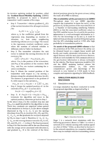
• Step 4: Assign the updated position of i as the A 2-stage simulation has been conducted to verify
centroid of ( + 1) across all j’s the proposed algorithm as depicted in Fig. 4.
,
( + 1) = mean[ ( + 1)].

,

• Step 5: If ( + 1) − ( ) < ℎ ,

terminate the algorithm and move to the
optimal position, otherwise go back to Step 1.
In the above steps, is the constant step size and
ℎ is a small threshold for the algorithm to stop.
These two constants are empirical values gained
from simulation in Section 6. In the above example
illustrated in Fig. 3, ⃗⃗⃗ , ⃗⃗⃗ , ⃗⃗⃗ are the moving
3
2
1
directions from to receivers , and .
3
1
0
2
, , are the gradients for receivers obtained
1 2 3 Fig. 4 – Simulation hierarchy
by in steps 1 and 2. Therefore, ⃗⃗⃗ ∙ , ⃗⃗⃗ ∙ ,
2
1
0
1
2
⃗⃗⃗ ∙ are the moving distance towards to , Stage 1 is a network level simulation with the
3
1
0
3
and , if = 1 in Step 3. The final movement following parameters shown in Table 1 to mimic a
3
2
in Step 4 for this iteration will be the one illustrated network of 21 vehicles moving with random speed
with the orange arrow annotated with direction ⃗⃗⃗ on a RoI of 450m * 450m, as described in Section 3.
0
and gradient . It is the centroid of the three In the network simulation, in a snapshot subframe,
there may be multiple vehicles transmitting, driven
0
© International Telecommunication Union, 2022 41