Page 68 - ITU Journal Future and evolving technologies Volume 2 (2021), Issue 4 – AI and machine learning solutions in 5G and future networks

ITU Journal on Future and Evolving Technologies, Volume 2 (2021), Issue 4

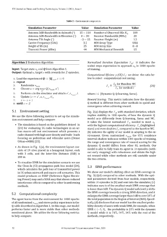
Table 2 – Environment components

Simulation Parameter Value Simulation Parameter Value
∘
Antenna 3dB‑Bandwidth in Azimuth ( ) 15 ∼ 110 Number of Observed UEs 0 100
∘
Antenna 3dB‑Bandwidth in Elevation ( ) 0 ∼ 30 Receiver Bandwidth (MHz) 20
∘
Antenna Tilt Angle ( ) −3 ∼ 15 Receiver Height (m) 1.5
Carrier Frequency (GHz) 3.5 MM Array Type URA
Height of BS (m) 25 MM Array Size 8×8
Transmit Power (dBm) 44 MM Mechanical Downtilt 15

Algorithm 2 Evaluation Algorithm Normalized Iteration Expectation ℐ : it indicates the

scaled steps expectation to approach in 1000 epochs
0
Input: Target state and Q from Algorithm 1. of training.
0
Output: Optimal , target with rewards for episodes.
Computational Ef icienc y (CE) ℰ : we de ine the ratio be‑
∗
1: Load the experienced Q ∶= [Q] , , ∶= 0 low to re lect computational cost saving:
2: repeat
E
3: Randomize ℰ ≜ ℐ for Baseline MC (20)
ℐ for method i
∗
′
4: Choose = arg ( , ) E
′
′
5: Perform in the simulator and obtain , , where ∈ {Dynamic Q, Q‑learning, Sarsa}.
′
6: Update ( ∶= , , , )

7: ← + 1 Reward Scoring: This metric indicates how the dynamic
8: until = Q method is different from other methods in speed and
convergence when achieving reward.
5.1 Environment setting Fig. 2(a) displays the ℐ with standard deviation, which

We use the three following metrics to set up the simula‑ implies stability in 1000 epochs, of how the dynamic Q
model acts differently from Q‑learning, Sarsa and MC.
tion environment and help compare:
It takes the lowest normalized ℐ needed to meet 0
• The simulation is based on the guidelines ined in with the highest computational ef iciency ℰ (highlighted
∗
[24] for evaluating 5G radio technologies in an ur‑ stars) and even doubles ℰ compared to the baseline MC.
∗
ban macro‑cell test environment which presents a (b) indicates the agility of our model in adapting to the en-
radio channel with high user density and tr ic loads vironment. Given randomized , the 95% con idence
focusing on pedestrian and vehicular users (Dense interval shadow indicates within 1000 epochs of training,
Urban‑eMBB) [25]. the range and convergence rate of reward scoring for the
dynamic Q model differs from other RL methods. Our
• As shown in Fig. 1(a), the environment layout con‑
model is able to fully train its agent in 10 episodes (with‑
sists of 19 sites placed in a hexagonal layout, each
out early stopping) with robustness and obtain the high‑
with 3 cells, and the Inter‑Site Distance (ISD) is
est reward while other methods are still unstable under
200 m.
the two criteria.
• To visualize SINR for the simulation scenario we use
the Close‑In (CI) propagation path loss model [26],
SINR performance
which calculates the path loss of transmitted power
in 5G urban microcell and macro‑cell scenarios. This We show our model’s shifting effect on SINR coverage in
model produces an RSRP (Reference Signal Receiv‑ Fig. 2(c)(d) compared to other methods. With the opti‑
ing Power) map and a SINR map that shows reduced mal parameters derived from four models, respectively,
interference effects compared to other beamforming within 10 episodes in (b) and sent into the simulator, (c)
methods. indicates ours is of the smallest weak SINR coverage that
is lower than 0dB. The dynamic Q model suf icientl y shifts
the SINR coverage towards a strong SINR direction, and it
5.2 Computational complexity
enlarges the SINR coverage larger than 0 dB to over 50% of
The agent learns from the environment for 1000 epochs the total population in the Region of Interest (ROI). Specif‑
of all randomized and stores policy experience in the ically, (d) discloses that our model has the smallest proba‑
Q‑table described in Algorithm 1. In this stage, our model bility density of users with weak SINR, for example, when
performs faster and is more stable than other methods SINR ∈ (−5, 0], the probability is 23% with the dynamic
mentioned above. We utilize the three following metrics Q model while it is 74%, 58%, 38% with the rest of the
to help compare: methods, respectively.

52 © International Telecommunication Union, 2021