Page 108 - Proceedings of the 2017 ITU Kaleidoscope

2017 ITU Kaleidoscope Academic Conference

{0, 1}, depending on the outcome of the similarity measure. in Table 2 so that distance apart can be derived. In computing
That is S f : C×C → {0, 1} ⊂ N and is based on correlation the distance measure to capture the information for the preva-
with other objects or features: lence threshold, our approach adopts key principles of basic
geometry and extends them to the current research in achiev-
(
1 if P f (C i ) = P f (C j ) ing the 2-D components for the day and time attributes. The
S f (C i , C j ) = location (loc) attribute typically has the longitude (long) and
0 otherwise
latitude (lat) as its (2-D) components (X, Y ), while that of
Definition 2. (Coherence) The coherence of a set of crime day and time is computed using the standard geometry con-
C i , C j is defined as the sum of their pairwise similarities cept.
F
X Table 2. A depiction of the 2-D components for determining
Coherence(C i , C j ) = S f (C i , C j ). (1)
prevalence characteristics
f=1
Geo Loc Day Time
Definition 3. (Significance Threshold (S)) The significance C 1 (long, lat) (x, y) (x, y)
threshold S for a set of crimes, C, in the feature space is (long, lat) (x, y) (x, y)
C 2
. . . .
defined as the coherence threshold for two crime objects C i . . . .
and C j to be considered similar. That is if the two crimes . . . .
exhibit sufficient related attributes in common, then we define
crime similarity (S) as follows:
More formally, P is set to the 3rd quartile among the set of
(
1 if Coherence(C i , C j ) ≥ S values computed in the following manner: Consider a crime
S(C i , C j ) = object C i ∈ C, we form the 6−component vector A us-
i
0 otherwise
ing the 2-D co-ordinates of P day (C i ), P loc (C i ), P time (C i ).
Thus,
The crime similarity for any non-null crime object refer-
i
ence(s) has the following properties: A = (P day (C i ), P loc (C i ), P time (C i )).
1. S(C i , C i ) = true (i.e. 1); [reflexive]. If Coherence(C i , C j ) exceeds S (the significance thresh-
old), we compute the 6D Euclidean distance d ij between A i
2. S(C i , C j ) = true ⇐⇒ S(C j , C i ) = true ; [symme- j
and A . If the distance is within range, that is not greater than
try].
the threshold P, then (C i , C j ) are connected in the similarity
0
graph. P is set to the 3rd quartile of the d ij s. on the advice
3. S(C i , C j ) ≥ 0; [non-negativity].
of crime experts.
4. S(C i , C j ) = 0, ⇐⇒ C i and C j are independent
Definition 4. (Similarity Graph) A similarity graph is an
[well-defined].
undirected graph G = (V, E), where V depicts the set of ver-
5. (S(C i , C j ) = 0) || (S(C i , C j ) = 1); [consistency]. tices, E depicts the set of edges, E = {{v i v j } : Λ(v i , v j ) ≥
S, (v i , v j ) ` P, v i , v j ∈ V, v i 6= v j }.
Our threshold is computed based on a sound mathematical
principle and crime expert recommendations. The signifi- F
X
cance and prevalence thresholds measure the interest similar- Λ(v i , v j ) = S f (v i , v j ). (2)
ity support, and helps to conceptualise the underlying graph-
f=1
ical structure, and ensures that a link ensues between two
crimes if and only if the support of the similarity attributes
is greater than or equal to parameters S(:= 5) and P. While
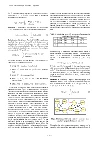
the parameter S come from crime intelligence experts as was Crime 9 Crime 7
also done in previous research [5], the coefficient P is a pa- Crime 3 Crime 1
rameter we learn from the data. The prevalence threshold
considers attributes relating to “day”, “time” and “location”
Crime 5
information of a crime incident. These features are consid- Crime 8 Crime 2
ered because of their potential characteristics in assisting the Crime 6 Crime 4
analysis as a series will happen within a close space-time
proximity. While the significance threshold helps to elimi-
nate the first level of uncertainty between two crime objects,
that is knowing whether the crime objects, say C i , C j , are Fig. 2. Identifying sufficiently connected nodes in a crime
sufficiently similar to be considered for further analysis, the similarity graph (red edges are min-cut)
prevalence characteristics (threshold P) further affirms the
proximity condition. In learning a suitable value for parame- The underlying crime incidents dependency structure can be
ter P, we consider the data set derived for analysis as shown modelled using a graphical approach as shown in Figure 2,

– 92 –