Page 214 - ITU Kaleidoscope 2016

2016 ITU Kaleidoscope Academic Conference

adaptation, and (ii) Heuristic Decision based Rate
 p'   q  (3)
 1 −  i  = 1 +  i 

i
i
 α L  X tp  θ L  ε t Adaptation (HDR) method is formulated and presented here.
 i = 1   i = 1 
i
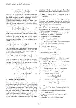
where L is the lag operator, α i is the autoregressive part 4.1 ARIMA Bitrate Based Adaptation (ABBA)
(Auto_Reg) and θ i is the moving average part (Mov_Avg) of Algorithm
the model linking the correlation between the successive
th
time windows under evaluation for the i packet. The sliding window size used for analysis can be
Now, the Auto_Reg polynomial would have a unitary root of
multiplicity d when applied to a non-linear stochastic process incremented using a constant factor inc_fac that could be
predefined to overcome the stationarity issues based on the
where the first order differencing of a characteristic equation
is non-stationary as sample data points taken into consideration.
ABBA Algorithm:
' d
 ' p   p −  (4)
 1− α i =  1− φ i 1 ( − ) L d Input: Bit Rates of packets for a Period of Time
 i L   i L  Output: Forecasted Bit Rate for the next sequence of packets
 i = 1   i = 1 
1. Start streaming of video content
The stationarity here refers to the time series bit rate based
model whose variance and auto correlation structures do not 2. Sample the data rate by choosing a sequence of packets
vary over time. 3. Initialize N, inc_factor, p, q, d, k for AIC.
Integrating polynomial (4) with the Moving Average 4. Compute µ r, µ s, µ t. // Calculate mean
component (Mov_Avg) [14] to determine the future 5. While (i<N) // Take N samples
sequence by factorization of p = p’ - d would give rise to 6. If (µ r = = µ s) //Test for stationarity
ARIMA model as
7. If (C xx(r,s) == C xx(r-1, s-1)) // C xx is the covariance
 p   q  8. N = N + inc_factor // Increment window size
 1 − φ  i 1 ( − L) d = 1 + θ  i (5)

 i L  X tp  i L  9. for i = 1 to m
 i = 1   i = 1 
10. Evaluate the Lag Operator
The ARIMA in (5) can be generalized by adding a stochastic
drift constant δ that denotes the change of average of bit rates ( ) = − −
in a continuously changing process that is modeled as a =1
regression drift constant given by 11. Evaluate the variance σ s and σ r
 p   q  ∑ =1 ( − ) 2
 1 −  φ  i 1 ( − L) d = δ + 1 + θ  i (6) =

 i L  X tp   i L  −1
 i = 1   i = 1 
12. Compute θ as stated in (1) // Moving Average
Now, the near future bit rates X tp and trend of bandwidth 13. for j=1 to q // q is no of sample points chosen
fluctuations can be predicted to notify the server so that it 14. Evaluate Auto_Corr = θ * L // Correlation
can adapt accordingly as in (7) that integrate the correlation
and variance into a form of regression. 14. if (Auto_Corr!=0)
15. Compute Φ as shown in (2) // Auto Regression
 q   p  d (7) 16. for k=1 to p

/
X tp = δ '+   1+ θ i L i   1− φ i L i  1 ( − ) L 17. Evaluate Auto_Var = Φ * L // Covariance

 i = 1   i = 1  18. if (Auto_Var>0)
 p  19. Compute the forecasted X tp using (7)
where ' = δδ /  1− φ L i 1 ( − ) L d (8) 20. Compute variance as shown
 i 
 i = 1  = ∑ =1 ( − ) 2

( ) − 1
4. ALGORITHM DEVELOPMENT 21. Calculate the Akaike Information Criteria
2
There is a need for a standard benchmark criterion to =log +
ascertain if the model predicts relatively accurate value and
in this context the Akaike Information Criteria (AIC) [15- 22. else
16], is embedded in the proposed ABBA algorithm which 23. N= N + inc_factor //Increment Window size
helps in fine-tuning the quality of prediction model. The AIC 24. end for
act as a quality gauge in mathematical models using 25. Find the p,q,d that corresponds to the maximum
statistical parameters that computes the quality of a single {AIC [i]} max in the array
model which is used as one of decision parameter. 26. Designate the optimal values for p, q, d and repeat
To compare the performance of the ABBA algorithm, two
existing approaches: (i) Buffer Switching Rate (BSR) from Step 9.
27. Repeat from step 5 until streaming occurs.

– 196 –